Reading Assignment 4
Deep Learning
Write your answers in a PDF and upload the document on Gradescope for submission. The due date is given on Gradescope.
Each question is worth 10 points. Please watch the videos and slides before answering these questions.
Each question starts with a reference to the corresponding video and slide deck in square brackets.
The next questions refer to slide deck “3.1 Loss function.”
- [3.1]. What is the common choice of activation function for regression tasks?
- [3.1]. Show that the Huber loss has a continuous derivative at $\lvert x \rvert = \delta$. Make sure that the signs are correct.
- [3.1]. Explain how a DNN can produce a probability vector $p_i$, $i = 1, \dots, n,$ given some real numbers $z_i,$ $i = 1, \dots, n.$
The next questions refer to slide deck “3.2 Cross-entropy”.
The maximum of the entropy $H(p) = - \sum_i p_i \ln p_i$ is achieved when $p_i$ is constant and $p_i = 1/n$; $n$ is the number of states. Let’s prove this result.
We want to maximize $H(p)$ under the constraint that $\sum_i p_i = 1$. The constraint $p_i \ge 0$ is actually not required to find the solution in this case.
To solve optimization problems under constraints, we can use the method of Lagrange multipliers. We define
$ H_1(p,\lambda) = - \sum_i p_i \ln p_i + \lambda (\sum_i p_i - 1) $
We can now maximize $H_1(p,\lambda)$ without having to worry about any constraint.
- [3.2]. Since $\partial H_1 / \partial \lambda = 0$ at the optimum, show that this implies that $\sum_i p_i = 1$ at the optimum.
- [3.2]. Calculate $\partial H_1 / \partial p_i$ in terms of $p_i$ and $\lambda$.
- [3.2]. Use the fact that $\partial H_1 / \partial p_i = 0$, for all $i$, at the optimum to show that all the $p_i$ are equal to each other (it is a uniform probability). Conclude that $p_i = 1/n$ using $\sum_i p_i = 1$. This is the value at which the maximum is achieved.
We can use the same method to find the minimum of the cross-entropy with respect to $q_i$.
We now use the following cost function with a Lagrange multiplier. The probability $p$ is now fixed for this problem.
$ H_2(q,\lambda) = - \sum_i p_i \ln q_i + \lambda (\sum_i q_i - 1) $
Don’t get confused between $p_i$ and $q_i$ in this expression.
As before, we can prove that at the point of minimum, $\sum_i q_i = 1$.
- [3.2]. Calculate $\partial H_2 / \partial q_i$ in terms of $p_i$, $q_i$, and $\lambda$.
- [3.2]. Show that $\partial H_2 / \partial q_i = 0$ implies that $q_i = p_i / \lambda$.
- [3.2]. Since $\sum_i q_i = \sum_i p_i = 1,$ conclude that $q_i = p_i$ when the cross-entropy is minimum.
The next questions refer to slide deck “3.3 TensorFlow loss functions”.
- [3.3]. Assume you use the
CategoricalCrossentropyloss function in TF. What constraints do you need to impose on the output $\hat{y}$ of the DNN so that the loss function is valid and meaningful? - [3.3]. Consider the hinge loss function and assume that $y = 1$ for some input $x$. Plot the loss function as a function of $\hat{y}$ the output of the DNN. Assume that $-\infty < \hat{y} < \infty$.
The next questions refer to slide decks “3.4 Backpropagation” and “3.5 Backpropagation formula”.
- [3.4]. Assume you have the vector $z = [0, \pi, 3\pi/2]$ and $\phi(x) = \cos(x)$. What is $\phi \odot z$ equal to?
- [3.4]. Assume that $y = a^T \phi \odot (w x + b)$ where $a$, $b$, and $x$ are vectors of size $n$, and $w$ is a scalar. Calculate $\partial y / \partial w$ (this is a scalar) and $\partial y / \partial b$ (this is a vector).
- [3.4]. Assume that $L = (y - a^T \tanh \odot (W x + b))^2 $ where $y$ is a scalar, $a$, $x$, and $b$ are vectors of size $n$, and $W$ is an $n \times n$ matrix.
tanhis the hyperbolic tangent function. Calculate $\partial L / \partial W$ (an $n \times n$ matrix) and $\partial L / \partial b$ (a column vector). Make sure you differentiate scalars, vectors, and matrices. - [3.5]. Assume we use the ReLU activation function for all layers. At some layer $k$, we have that $[W^{(k)} a^{(k-1)} + b^{(k)}]_i < 0$, for all $i$. Show that $\partial y / \partial W^{(l)} = 0$ for all $1 \le l \le k+1$. Note that $l = k+1$ is included.
- [3.5]. Summarize the steps required to compute $\partial y / \partial W^{(k)}$ using a forward and backward pass in the backpropagation algorithm.
The next questions refer to slide deck “3.6 Learning rate for training.”
- [3.6]. How many steps does it take to minimize a loss function that is quadratic if you can compute the gradient and the inverse of the Hessian matrix?
- [3.6]. Take a loss function that is quadratic, with $H$ symmetric positive definite. Prove that, with an appropriate change of variable, the update rule can be written as a decoupled set of equations: $\Delta Z = - \alpha \Lambda Z$, where $\Lambda$ is a diagonal matrix.
- [3.6]. Describe the convergence of a gradient-based method when the ratio $\lambda_1 / \lambda_n$ is close to 1 and when this ratio is large.
The next question refers to slide deck “3.7 Empirical method for learning rate.”
- [3.7]. Write a few lines of Python code to implement a learning rate schedule in which the learning rate decays like 1/epoch. Use a formula like
initial_learning_rate / (1 + decay_rate * floor(step / decay_step))
You need to implement a Python function that returns the learning rate (following the example in the slides), then one line to call keras.callbacks.LearningRateScheduler(...) and the call to dnn.fit(...) using callbacks=[...].
TensorFlow documentation: LearningRateScheduler, Keras optimizers schedules
The next question refers to slide deck “3.8 Overfitting.”
Consider the figure below

The figure contains 8 points. We can fit a polynomial of order 7 through all these data points.
- [3.8]. How accurate is this polynomial fitting procedure if we want to make predictions? What polynomial would you fit through this data in order to make accurate predictions? Explain how this is related to the concept of overfitting.
Extra reading relevant to this problem: Overfitting
The next questions refer to slide deck “3.9 DNN initializers.”
- [3.9]. Explain the problem of vanishing gradient in deep learning.
- [3.9]. Using a simple argument, explain why the variance of the weights $w_{ij}$, during initialization, should depend on the size of the layers.
- [3.9]. Assume that layer $i$ has 4 nodes and layer $i+1$ has 5 nodes. How would you initialize the weight matrix that connects layers 4 and 5 using the Glorot-Bengio formula given in the slides?
Additional reading: Understanding the difficulty of training deep feedforward neural networks by Glorot and Bengio. See their famous equation (16) on p. 253.
The next questions refer to slide deck “3.10 Regularization.”
- [3.10]. Write a few lines of Python, with TensorFlow, to define a dense fully connected layer with 16 output nodes, an initializer for the weights that sets all the weights equal to the constant 1/4, and an l1 regularizer on the weights with parameter $\lambda = 0.001$.
Relevant documentation in TensorFlow: regularizers, initializers, constant initializer.
See also the section “Configure the layers” in Keras overview for examples.
- [3.10]. Explain the difference between l1 and l2 regularization. If you want a sparser network, which regularization would you pick? Which type of regularization is typically easier to solve for numerically?
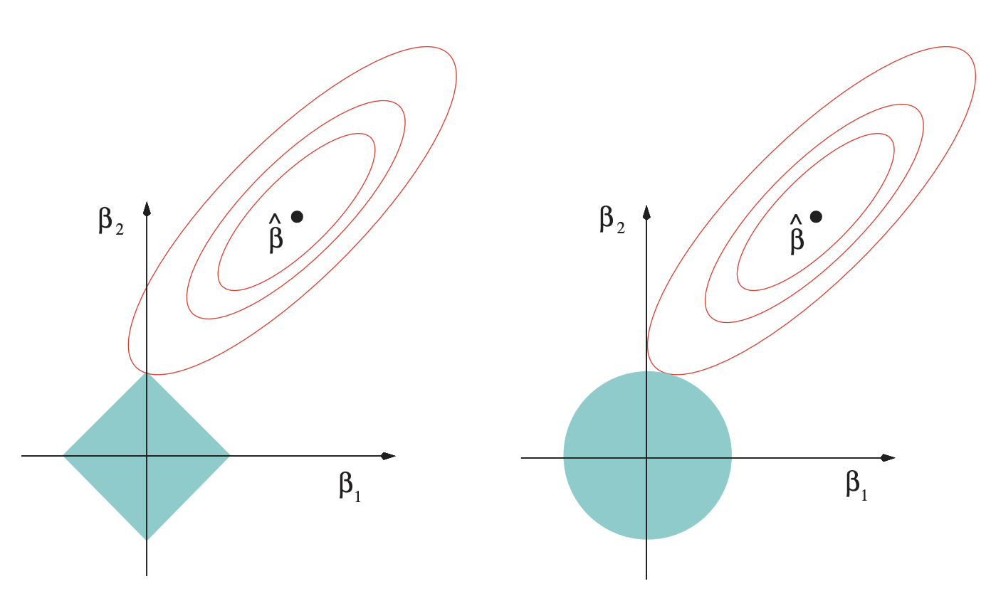
For additional reading, please check The Elements of Statistical Learning by Stanford professors Trevor Hastie, Robert Tibshirani, and Jerome Friedman. The book is accessible online. You can check section 3.4.3 which compares l1 and l2 regularizations. The loss function in this case is quadratic. The unknowns are $\beta$. l2 is described in section 3.4.1. It’s the ridge regression method. See Eqns. (3.41) and (3.42) p. 63. Lasso corresponds to the l1 regularization. See Eqns. (3.51) and (3.52) in Section 3.4.2, p. 68. Section 3.4.3 compares these methods. Table 3.4, p. 71, shows the optimal $\beta$ selected by each method. “Best subset” tries to pick the best $M$ coefficients for the fit and zeros out all the others. This is a possible regularization method. You can see how Lasso tends to zero out coefficients.
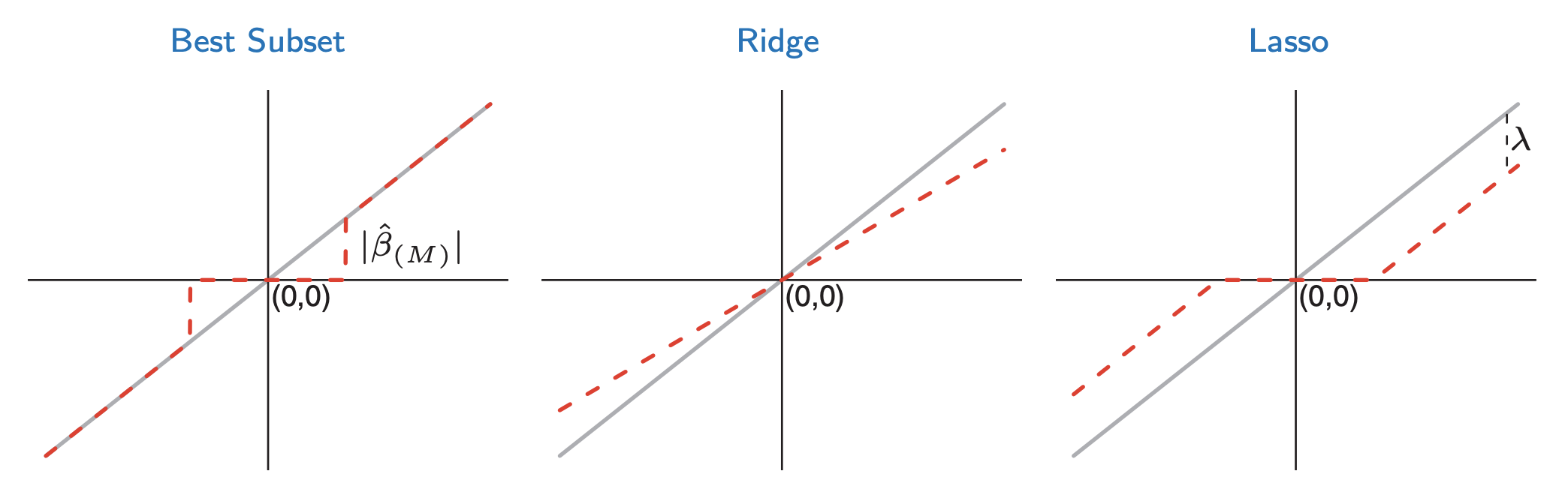
The $x$-axis is $\beta$ without regularization and the $y$-axis is $\beta$ with regularization. Ridge is l2 and Lasso is l1. Small values of $\beta$ are zeroed out by Lasso. The grey line is the solution without regularization.
Fig. 3.11, p. 71, shows the quadratic loss function (red ellipses in the top right). The regularizing constraints are shown as a blue square (left, l1) and a circle (right, l2). This figure illustrates why l1 regularization tends to lead to solutions that are sparse.